Loads Spatial Data Sets Related to China

The geocn package provides various commonly used spatial data related to Chinese regions in the R programming environment. This vignette presents a quick intro to geocn.

Available data sets

The geocn package covers 19 spatial data sets, including a variety of relevant data from both the global and Chinese regions. You can view what data sets are available using the list_geocn() function.

library(sf)
## Linking to GEOS 3.10.2, GDAL 3.4.1, PROJ 8.2.1; sf_use_s2() is TRUE
library(geocn)
library(ggplot2)

datasets_geocn = list_geocn()
datasets_geocn
## # A tibble: 19 × 2
##    functions               results                                              
##    <chr>                   <chr>                                                
##  1 load_world_country      Global Country Boundaries                            
##  2 load_world_continent    Global Continents                                    
##  3 load_world_coastline    Global Coastlines                                    
##  4 load_world_ocean        Global Oceans                                        
##  5 load_world_lake         Global Lakes                                         
##  6 load_world_river        Global Rivers                                        
##  7 load_cn_province        Province-Level Administrative Units in China         
##  8 load_cn_city            City-Level Administrative Units in China             
##  9 load_cn_county          County-Level Administrative Units in China           
## 10 load_cn_border          China's Land Border Line and the 10-dash line of the…
## 11 load_cn_landborder      China's Land Border                                  
## 12 load_cn_coastline       Coastline of China                                   
## 13 load_cn_tenline         10-dash line of the South China Sea                  
## 14 load_cn_landcoast       China's Land Border and Coastline                    
## 15 load_tibetan_plateau    Tibetan Plateau Boundary                             
## 16 load_loess_plateau      Loess Plateau Boundary                               
## 17 load_yangtze_basin      Yangtze River Basin Boundary                         
## 18 load_yellow_river_basin Yellow River Basin Boundary                          
## 19 load_weihe_basin        Weihe River Basin Boundary

Commonly Used CRS for Drawing Maps of China

The load_cn_alberproj() function can be used to obtain the CRS information available in the sf and terra packages. By default, it returns in sf format. However, you can specify the return format through the output parameter.

albers = load_cn_alberproj()

province = load_cn_province()
## Warning in CPL_read_ogr(dsn, layer, query, as.character(options), quiet, : GDAL
## Message 1: organizePolygons() received a polygon with more than 100 parts.  The
## processing may be really slow.  You can skip the processing by setting
## METHOD=SKIP.
ggplot(data = province) +
  geom_sf(fill = 'grey90', color = 'grey') +
  theme_bw()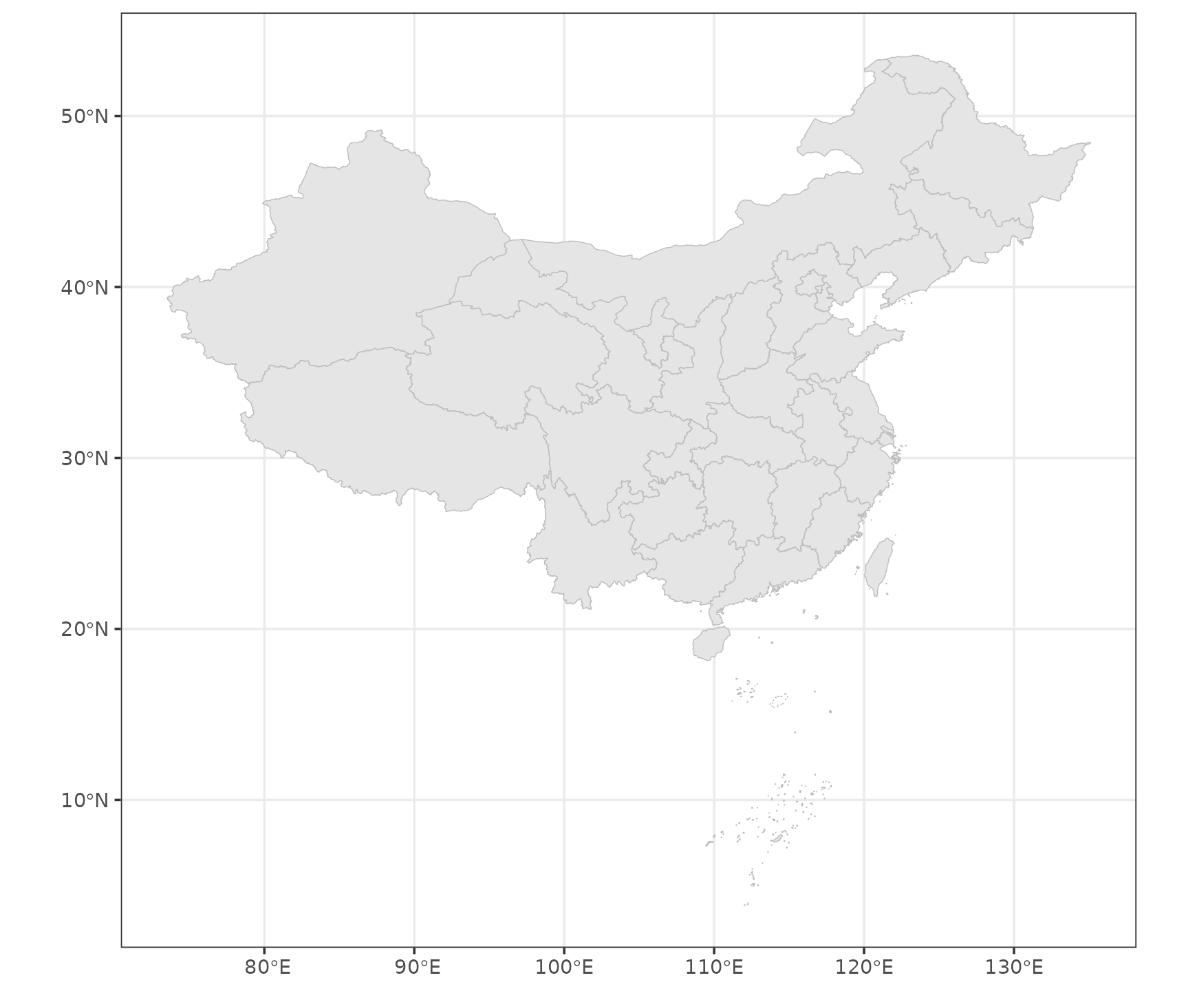

province_albers = st_transform(province,albers)
ggplot(data = province_albers) +
  geom_sf(fill = 'grey90', color = 'grey') +
  theme_bw()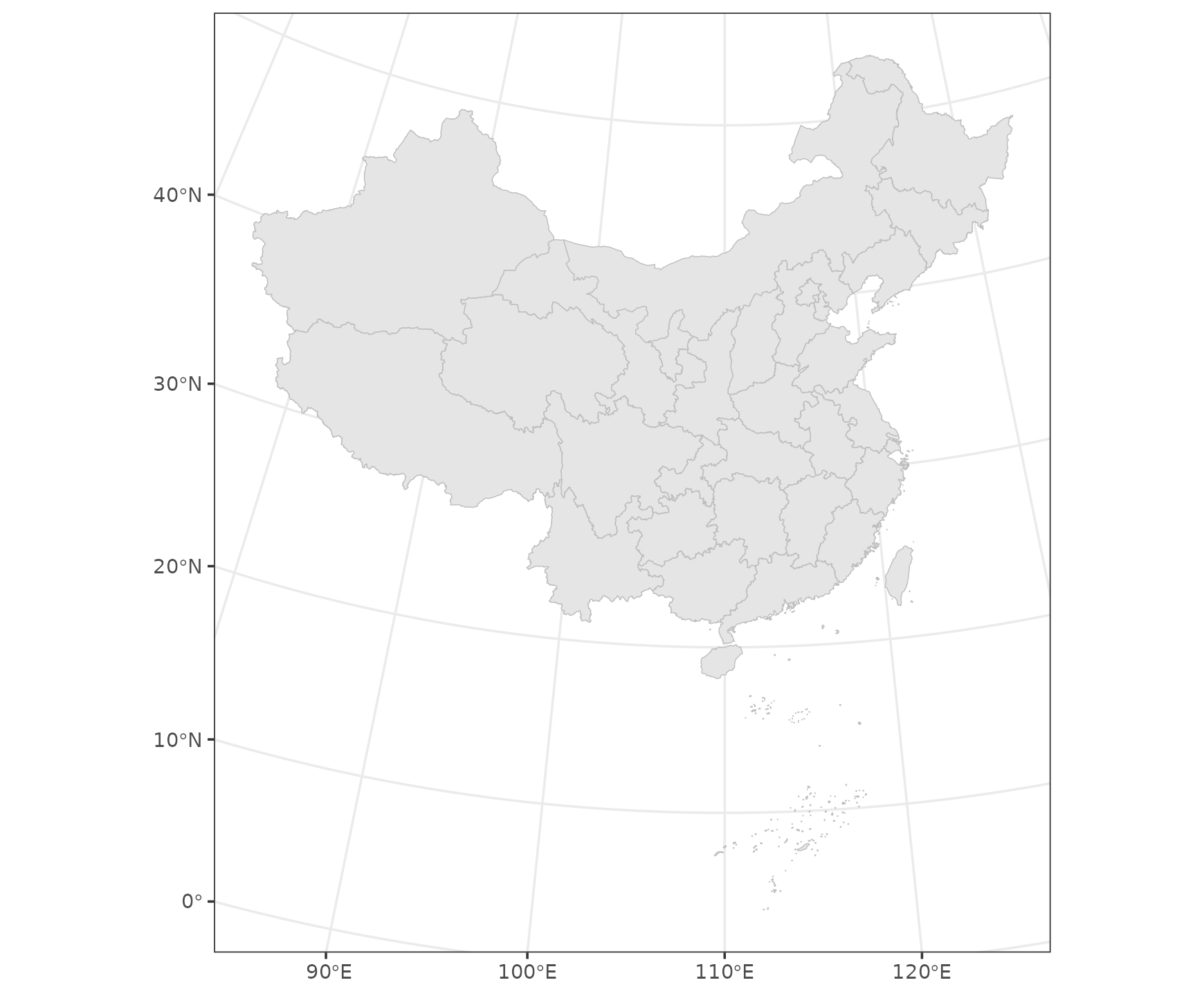

Region-specific CRS Transformation in China

This section primarily focuses on the conversion between the GCJ02, BD09, and WGS84 coordinate systems. The geocn provides st_transform_cn() function to achieve the conversion. You need to input the longitude and latitude coordinate vectors to be transformed as function parameters lon and lat, and specify the CRS before transformation and the CRS to be transformed. Please note that in the st_transform_cn() function, the from and to parameters respectively refer to wgs, gcj, bd for WGS84, GCJ02, BD09 coordinate systems. Default Conversion from GCJ02 to WGS84.

lon = c(126.626510,126.625261,126.626378,126.626541,126.626721,126.627732,126.626510)
lat = c(45.731596,45.729834,45.729435,45.729676,45.729604,45.730915,45.731596)
st_transform_cn(lon,lat)
## # A tibble: 7 × 2
##     lon   lat
##   <dbl> <dbl>
## 1  127.  45.7
## 2  127.  45.7
## 3  127.  45.7
## 4  127.  45.7
## 5  127.  45.7
## 6  127.  45.7
## 7  127.  45.7