We demonstrate the necessity of the spatial explicit discretization
(discretization with spatial soft constraints) method using the
Depression.csv data from the gdverse package.
In this analysis, we select Depression_prevalence as the
dependent variable \(Y\) and
PopulationDensity as the independent variable \(X\). \(X\)
is randomly shuffled, and the q-value is calculated using both
discretization methods that do and do not account for spatial soft
constraints, with the process repeated 5000 times. We selected
hierarchical clustering with spatial soft constraints and hierarchical
clustering without spatial soft constraints method to represent explicit
and implicit spatial discretization, respectively. At the same time,
natural breaks method and robust discretization are used as the control
in this experiment. The hierarchical clustering with spatial soft
constraints method, hierarchical clustering without spatial soft
constraints method and the natural breaks method were implemented using
the sdsfun package, and the robust discretization is
implemented by gdverse package. In subsequent analyses, all
discretization methods applied will discretize the dataset into five
strata for the calculation of the q-values.
Install necessary R packages
install.packages("gdverse",dep = TRUE)
# install.packages("devtools")
devtools::install_github("stscl/sesp",build_vignettes = TRUE,dep = TRUE)
The spatial autocorrelation of the example data
dt = system.file('extdata/Depression.csv',package = 'gdverse') |>
  readr::read_csv() |>
  sf::st_as_sf(coords = c('X','Y'), crs = 4326) |>
  dplyr::select(y = Depression_prevelence,
                x = PopulationDensity)
## Rows: 1072 Columns: 13
## ── Column specification ───────────────────────────────────────────────────────────────────────────
## Delimiter: ","
## dbl (13): X, Y, Depression_prevelence, PopulationDensity, Population65, NoHealthInsurance, Neig...
##
## ℹ Use `spec()` to retrieve the full column specification for this data.
## ℹ Specify the column types or set `show_col_types = FALSE` to quiet this message.

sdsfun::moran_test(dt)
## *** global moran test| Variable | MoranI | EI | VarI | zI | pI |
|---|---|---|---|---|---|
| y | 0.339557*** | -0.0009337 | 0.0003192 | 19.06 | 2.892e-81 |
| x | 0.365364*** | -0.0009337 | 0.0003192 | 20.5 | 1.052e-93 |
Q values corresponding to spatial implicit discretization
geom = sf::st_geometry(dt)
y = dt$y
x = dt$x

x_naturaldisc = sdsfun::discretize_vector(x,5,method = "natural")
x_hclustdisc = sdsfun::hclustgeo_disc(dplyr::select(dt,x),5,alpha = 0)
x_robustdisc = gdverse::robust_disc(y ~ .,
                                    data = tibble::tibble(y = y,x = x),
                                    discnum = 5, cores = 1) |>
  dplyr::pull(1) |>
  as.factor() |>
  as.integer()
qv_naturaldisc = gdverse::factor_detector(y,x_naturaldisc)[[1]]
qv_naturaldisc
## [1] 0.07985365
qv_hclustdisc = gdverse::factor_detector(y,x_hclustdisc)[[1]]
qv_hclustdisc
## [1] 0.07315131
qv_robustdisc = gdverse::factor_detector(y,x_robustdisc)[[1]]
qv_robustdisc
## [1] 0.1199684
A Monte Carlo simulation experiment demonstrating the necessity of spatial explicit discretization
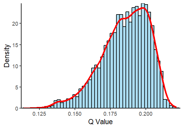
In the repeated experiment, \(X\) is shuffled 5000 times, and the global Moran’s I of the original independent variable \(X\) serves as the degree of spatial soft constraint (0.365 in this case). Subsequently, the q-values for each simulation round is computed.
mc_simq = \(times = 1000, cores = 6){
  doclust = FALSE
  if (inherits(cores, "cluster")) {
    doclust = TRUE
  } else if (cores > 1) {
    doclust = TRUE
    cores = parallel::makeCluster(cores)
    on.exit(parallel::stopCluster(cores), add = TRUE)
  }

  calcul_q = \(n_sim) {
    x_sim = sample(x)
    x_sim = sf::st_set_geometry(tibble::tibble(x_sim = x_sim),geom)
    g = sdsfun::moran_test(x_sim)
    moran = dplyr::pull(g$result,2)
    moran_p = dplyr::pull(g$result,6)
    x_sed = sdsfun::hclustgeo_disc(x_sim, n = 5, alpha = 0.365)
    qv1 = gdverse::factor_detector(y,x_sed)[[1]]
    res = tibble::tibble(qv_sed = qv1, moran = moran,
                         moran_p = moran_p)
    return(res)
  }

  if (doclust) {
    parallel::clusterExport(cores,varlist = c("geom","x","y"))
    out_g = parallel::parLapply(cores,seq(1,times,by = 1),calcul_q)
    out_g = tibble::as_tibble(do.call(rbind, out_g))
  } else {
    out_g = purrr::map_dfr(seq(1,times,by = 1),calcul_q)
  }
  return(out_g)
}
qv = mc_simq(times = 5000, cores = 12)
qv
## # A tibble: 5,000 × 3
##    qv_sed    moran moran_p
##     <dbl>    <dbl>   <dbl>
##  1  0.177  0.00782   0.312
##  2  0.136 -0.00580   0.607
##  3  0.210  0.00788   0.311
##  4  0.180  0.0145    0.194
##  5  0.180  0.0177    0.148
##  6  0.199  0.00956   0.278
##  7  0.174 -0.00721   0.637
##  8  0.195 -0.0190    0.844
##  9  0.200 -0.00940   0.682
## 10  0.167  0.0140    0.202
## # ℹ 4,990 more rows
ggplot2::ggplot(data = qv, ggplot2::aes(x = qv_sed)) +
  ggplot2::geom_histogram(ggplot2::aes(y = ggplot2::after_stat(density)),
                          bins = 50, fill = "skyblue",
                          color = "black", alpha = 0.7) +
  ggplot2::geom_density(color = "red", linewidth = 1.2) +
  ggplot2::scale_x_continuous(expand = c(0.01, 0)) +
  ggplot2::scale_y_continuous(expand = c(0, 0)) +
  ggplot2::labs(x = "Q Value",
                y = "Density") +
  ggplot2::theme_classic()
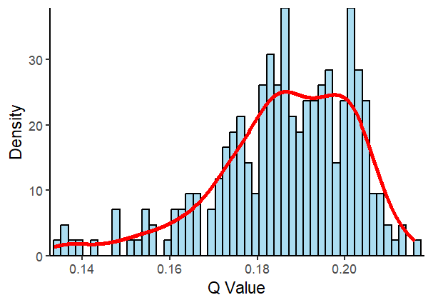
We selected simulated q-values that are more consistent with the actual situation, specifically those for which the global Moran’s I of the permuted data is statistically significant (p-value < 0.05) and greater than zero.
qv_sign = dplyr::filter(qv,moran>=0&moran_p<=0.05)
qv_sign
## # A tibble: 252 × 3
##    qv_sed  moran   moran_p
##     <dbl>  <dbl>     <dbl>
##  1  0.204 0.0308 0.0376
##  2  0.175 0.0304 0.0395
##  3  0.171 0.0325 0.0305
##  4  0.189 0.0523 0.00143
##  5  0.197 0.0296 0.0437
##  6  0.151 0.0423 0.00774
##  7  0.175 0.0388 0.0131
##  8  0.191 0.0328 0.0294
##  9  0.206 0.0331 0.0285
## 10  0.197 0.0720 0.0000222
## # ℹ 242 more rows
ggplot2::ggplot(data = qv_sign, ggplot2::aes(x = qv_sed)) +
  ggplot2::geom_histogram(ggplot2::aes(y = ggplot2::after_stat(density)),
                          bins = 50, fill = "skyblue",
                          color = "black", alpha = 0.7) +
  ggplot2::geom_density(color = "red", linewidth = 1.2) +
  ggplot2::scale_x_continuous(expand = c(0.01, 0)) +
  ggplot2::scale_y_continuous(expand = c(0, 0)) +
  ggplot2::labs(x = "Q Value",
                y = "Density") +
  ggplot2::theme_classic()
The q-value derived from classifying into five categories using the natural breaks method is 0.07985, while the q-value from five-category hierarchical clustering without spatial constraints is 0.07315. In comparison, the q-value obtained through robust discretization into five categories is 0.11997. In the Monte Carlo simulation experiment, the q-values range from 0.1138 to 0.22158. Among randomized simulations that best align with actual conditions, the q-value range spans from 0.13359 to 0.21584. These results indicate that spatially implicit discretization tends to underestimate the q-value of the variable under moderate spatial autocorrelation, highlighting the importance of spatially explicit discretization. The results also reveal that robust discretization, which accounts for the relationship between independent and dependent variables, can effectively reduce the q-value estimation bias introduced by spatially implicit discretization methods. However, it still underestimates the q-value by approximately 35.2584%. This highlights the need for a spatially explicit discretization approach that fully considers the relationship between independent and dependent variables to more accurately capture the impact of spatial dependence on discretization.
