State Space Reconstruction

Wenbo Lv

Last update: 2025-11-01
Last run: 2025-11-07

Methodological Background

Takens theory proves that for a dynamical system \(\phi\), if its trajectory converges to an attractor manifold \(M\)—a bounded and invariant set of states—then there exists a smooth mapping between the system \(\phi\) and its attractor \(M\). Consequently, the time series observations of \(\phi\) can be used to reconstruct the structure of \(M\) through delay embedding.

According to the generalized embedding theorem, for a compact \(d\)-dimensional manifold \(M\) and a set of observation functions \(\langle h_1, h_2, \ldots, h_L \rangle\), the mapping \(\psi_{\phi,h}(x) = \langle h_1(x), h_2(x), \ldots, h_L(x) \rangle\) is an embedding of \(M\) when \(L \geq 2d + 1\). Here, embedding refers to a one-to-one map that resolves all singularities of the original manifold. The observation functions \(h_i\) can take the form of time-lagged values from a single time series, lags from multiple time series, or even completely distinct measurements. The former two are simply special cases of the third.

This embedding framework can be extended to spatial cross-sectional data, which lack temporal ordering but are observed over a spatial domain. In this context, the observation functions can be defined using the values of a variable at a focal spatial unit and its surrounding neighbors (known as spatial lags in spatial statistics). Specifically, for a spatial location \(s\), the embedding can be written as:

\[ \psi(x, s) = \langle h_s(x), h_{s(1)}(x), \ldots, h_{s(L-1)}(x) \rangle, \]

where \(h_{s(i)}(x)\) denotes the observation function of the \(i\)-th order spatial lag unit relative to \(s\). These spatial lags provide the necessary diversity of observations for effective manifold reconstruction. In practice, if a given spatial lag order involves multiple units, summary statistics such as the mean or directionally-weighted averages can be used as the observation function to maintain a one-to-one embedding.

Usage examples

An example of spatial lattice data

Load the spEDM package and its county-level population density data:

library(spEDM)

popd_nb = spdep::read.gal(system.file("case/popd_nb.gal",package = "spEDM"))
## Warning in spdep::read.gal(system.file("case/popd_nb.gal", package = "spEDM")): neighbour
## object has 4 sub-graphs
popd = readr::read_csv(system.file("case/popd.csv",package = "spEDM"))
## Rows: 2806 Columns: 7
## ── Column specification ───────────────────────────────────────────────────────────────────────
## Delimiter: ","
## dbl (7): lon, lat, popd, elev, tem, pre, slope
## 
## ℹ Use `spec()` to retrieve the full column specification for this data.
## ℹ Specify the column types or set `show_col_types = FALSE` to quiet this message.
popd_sf = sf::st_as_sf(popd, coords = c("lon","lat"), crs = 4326)
popd_sf
## Simple feature collection with 2806 features and 5 fields
## Geometry type: POINT
## Dimension:     XY
## Bounding box:  xmin: 74.9055 ymin: 18.2698 xmax: 134.269 ymax: 52.9346
## Geodetic CRS:  WGS 84
## # A tibble: 2,806 × 6
##     popd  elev   tem   pre slope          geometry
##  * <dbl> <dbl> <dbl> <dbl> <dbl>       <POINT [°]>
##  1  780.     8  17.4 1528. 0.452 (116.912 30.4879)
##  2  395.    48  17.2 1487. 0.842 (116.755 30.5877)
##  3  261.    49  16.0 1456. 3.56  (116.541 30.7548)
##  4  258.    23  17.4 1555. 0.932  (116.241 30.104)
##  5  211.   101  16.3 1494. 3.34   (116.173 30.495)
##  6  386.    10  16.6 1382. 1.65  (116.935 30.9839)
##  7  350.    23  17.5 1569. 0.346 (116.677 30.2412)
##  8  470.    22  17.1 1493. 1.88  (117.066 30.6514)
##  9 1226.    11  17.4 1526. 0.208 (117.171 30.5558)
## 10  137.   598  13.9 1458. 5.92  (116.208 30.8983)
## # ℹ 2,796 more rows

Embedding the variable popd from county-level population density:

v = spEDM::embedded(popd_sf,"popd",E = 10)
v[1:5,c(4,5,10)]
##           [,1]     [,2]      [,3]
## [1,]  962.7204 1664.756 1581.4351
## [2,]  919.6000 2408.766 1494.8241
## [3,] 1435.0165 1958.686  813.9077
## [4,] 1488.2727 2066.748 1216.6986
## [5,] 2326.8429 1290.188 1038.3864

plot3D::scatter3D(v[,4], v[,5], v[,10], colvar = NULL, pch = 19,
                  col = "red", theta = 45, phi = 10, cex = 0.35,
                  bty = "f", clab = NA, tickmarks = FALSE)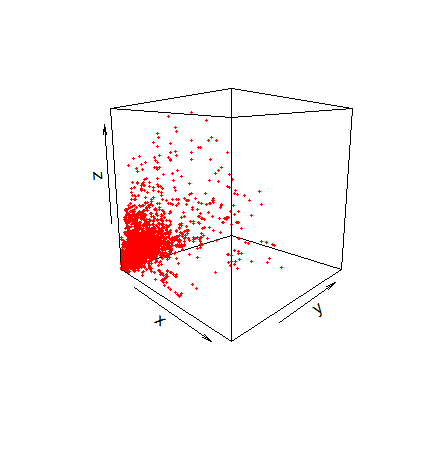

Figure 1. The reconstructed shadow manifolds for the variable popd.

An example of spatial grid data

Load the spEDM package and its farmland npp data:

library(spEDM)

npp = terra::rast(system.file("case/npp.tif", package = "spEDM"))
npp
## class       : SpatRaster 
## size        : 404, 483, 5  (nrow, ncol, nlyr)
## resolution  : 10000, 10000  (x, y)
## extent      : -2625763, 2204237, 1877078, 5917078  (xmin, xmax, ymin, ymax)
## coord. ref. : CGCS2000_Albers 
## source      : npp.tif 
## names       :      npp,        pre,      tem,      elev,         hfp 
## min values  :   164.00,   384.3409, -47.8194, -122.2004,  0.03390418 
## max values  : 16606.33, 23878.3555, 263.6938, 5350.4902, 44.90312195

Embedding the variable npp from farmland npp data:

r = spEDM::embedded(npp,"npp",E = 5,tau = 20)
r[which(!is.na(r),arr.ind = T)[1:5],1:3]
##          [,1]     [,2]     [,3]
## [1,] 2896.833 2933.926 2898.288
## [2,] 3664.286 3071.789 3003.966
## [3,] 3317.337 3090.832 2973.627
## [4,] 3196.011 3107.388 2942.477
## [5,] 3329.188 3080.360 2892.083

plot3D::scatter3D(r[,1], r[,2], r[,3], colvar = NULL, pch = 19,
                  col = "#e77854", theta = 45, phi = 10, cex = 0.01,
                  bty = "f", clab = NA, tickmarks = FALSE)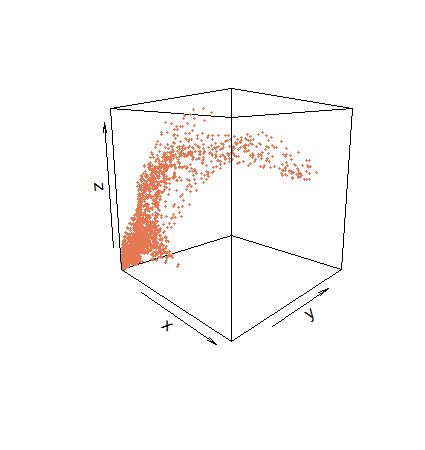

Figure 2. The reconstructed shadow manifolds for the variable npp.