Geographical Convergent Cross Mapping
Wenbo Lv
Last
update: 2025-11-25
Last run: 2025-11-30
Source: Last run: 2025-11-30
vignettes/GCCM.Rmd
GCCM.RmdMethodological Background
Let \(Y = \{y_i\}\) and \(X = \{x_i\}\) be the two spatial cross sectional variable, where \(i = 1, 2, \dots, n\) denotes spatial units (e.g., regions or grid cells), the shadow manifolds of \(X\) can be constructed using the different spatial lag values of all spatial units:
\[ M_{x} = \begin{bmatrix} S_{(\tau)}(x_1) & S_{(2\tau)}(x_1) & \cdots & S_{(E\tau)}(x_1) \\ S_{(\tau)}(x_2) & S_{(2\tau)}(x_2) & \cdots & S_{(E\tau)}(x_2) \\ \vdots & \vdots & \ddots & \vdots \\ S_{(\tau)}(x_n) & S_{(2\tau)}(x_n) & \cdots & S_{(E\tau)}(x_n) \end{bmatrix} \]
Here, \(S_{(j)}(x_i)\) denotes the \(j\) th-order spatial lag value of spatial unit \(i\), \(\tau\) is the step size for the spatial lag order, and \(E\) is the embedding dimension and \(M_{x}\) corresponds to the shadow manifolds of \(X\).
With the reconstructed shadow manifolds \(M_{x}\), the state of Y can be predicted with the state of X through
\[ \hat{Y}_s \mid M_x = \sum\limits_{i=1}^k \left(\omega_{si}Y_{si} \mid M_x \right) \]
where \(s\) represents a spatial unit at which the value of \(Y\) needs to be predicted, \(\hat{Y}_s\) is the prediction result, \(k\) is the number of nearest neighbors used for prediction, \(si\) is the spatial unit used in the prediction, \(Y_{si}\) is the observation value of \(Y\) at \(si\). \(\omega_{si}\) is the corresponding weight defined as:
\[ \omega_{si} \mid M_x = \frac{weight \left(\psi\left(M_x,s_i\right),\psi\left(M_x,s\right)\right)}{\sum_{i=1}^{L+1}weight \left(\psi\left(M_x,s_i\right),\psi\left(M_x,s\right)\right)} \]
where \(\psi(M_x, s_i)\) is the state vector of spatial unit \(s_i\) in the shadow manifold \(M_x\), and \(weight (\ast, \ast)\) is the weight function between two states in the shadow manifold, defined as:
\[ weight \left(\psi\left(M_x,s_i\right),\psi\left(M_x,s\right)\right) = \exp \left(- \frac{dis \left(\psi\left(M_x,s_i\right),\psi\left(M_x,s\right)\right)}{dis \left(\psi\left(M_x,s_1\right),\psi\left(M_x,s\right)\right)} \right) \]
where \(\exp\) is the exponential function and \(dis \left(\ast,\ast\right)\) represents the distance function between two states in the shadow manifold defined as:
\[ dis \left( \psi(M_x, s_i), \psi(M_x, s) \right) = \frac{1}{E} \sum_{m=1}^{E} \left| \psi_m(M_x, s_i) - \psi_m(M_x, s) \right| \]
where \(dis \left( \psi(M_x, s_i), \psi(M_x, s) \right)\) denotes the average absolute difference between corresponding elements of the two state vectors in the shadow manifold \(M_x\), \(E\) is the embedding dimension, and \(\psi_m(M_x, s_i)\) is the \(m\)-th element of the state vector \(\psi(M_x, s_i)\).
The skill of cross-mapping prediction \(\rho\) is measured by the Pearson correlation coefficient between the true observations and corresponding predictions, and the confidence interval of \(\rho\) can be estimated based the \(z\)-statistics with the normal distribution:
\[ \rho = \frac{Cov\left(Y,\hat{Y}\mid M_x\right)}{\sqrt{Var\left(Y\right) Var\left(\hat{Y}\mid M_x\right)}} \]
\[ t = \rho \sqrt{\frac{n-2}{1-\rho^2}} \]
where \(n\) is the number of observations to be predicted, and
\[ z = \frac{1}{2} \ln \left(\frac{1+\rho}{1-\rho}\right) \]
The prediction skill \(\rho\) varies by setting different sizes of libraries, which means the quantity of observations used in reconstruction of the shadow manifold. We can use the convergence of \(\rho\) to infer the causal associations. For GCCM, the convergence means that \(\rho\) increases with the size of libraries and is statistically significant when the library becomes largest.
\[ \rho_{x \to y} = \lim_{L \to \infty} cor \left( Y,\hat{Y}\mid M_x \right) \]
where \(\rho_{x \to y}\) is the correlation after convergence, used to measure the causation effect from \(Y\) to \(X\), despite the notation suggesting the reverse direction.
Usage examples
An example of spatial lattice data
Load the spEDM package and its county-level population
density data:
library(spEDM)

popd_nb = spdep::read.gal(system.file("case/popd_nb.gal",package = "spEDM"))
## Warning in spdep::read.gal(system.file("case/popd_nb.gal", package = "spEDM")):
## neighbour object has 4 sub-graphs
popd = readr::read_csv(system.file("case/popd.csv",package = "spEDM"))
## Rows: 2806 Columns: 7
## ── Column specification ────────────────────────────────────────────────────────
## Delimiter: ","
## dbl (7): lon, lat, popd, elev, tem, pre, slope
##
## ℹ Use `spec()` to retrieve the full column specification for this data.
## ℹ Specify the column types or set `show_col_types = FALSE` to quiet this message.
popd_sf = sf::st_as_sf(popd, coords = c("lon","lat"), crs = 4326)
popd_sf
## Simple feature collection with 2806 features and 5 fields
## Geometry type: POINT
## Dimension:     XY
## Bounding box:  xmin: 74.9055 ymin: 18.2698 xmax: 134.269 ymax: 52.9346
## Geodetic CRS:  WGS 84
## # A tibble: 2,806 × 6
##     popd  elev   tem   pre slope          geometry
##  * <dbl> <dbl> <dbl> <dbl> <dbl>       <POINT [°]>
##  1  780.     8  17.4 1528. 0.452 (116.912 30.4879)
##  2  395.    48  17.2 1487. 0.842 (116.755 30.5877)
##  3  261.    49  16.0 1456. 3.56  (116.541 30.7548)
##  4  258.    23  17.4 1555. 0.932  (116.241 30.104)
##  5  211.   101  16.3 1494. 3.34   (116.173 30.495)
##  6  386.    10  16.6 1382. 1.65  (116.935 30.9839)
##  7  350.    23  17.5 1569. 0.346 (116.677 30.2412)
##  8  470.    22  17.1 1493. 1.88  (117.066 30.6514)
##  9 1226.    11  17.4 1526. 0.208 (117.171 30.5558)
## 10  137.   598  13.9 1458. 5.92  (116.208 30.8983)
## # ℹ 2,796 more rows
Determining optimal embedding dimension:
spEDM::simplex(popd_sf, "pre", "pre", E = 2:10, k = 12)
## The suggested E,k,tau for variable pre is 3, 12 and 1
spEDM::simplex(popd_sf, "popd", "popd", E = 2:10, k = 12)
## The suggested E,k,tau for variable popd is 9, 12 and 1
Run GCCM:
startTime = Sys.time()
pd_res = spEDM::gccm(data = popd_sf, cause = "pre", effect = "popd",
                     libsizes = seq(100, 2800, by = 200),
                     E = c(3,9), k = 12, nb = popd_nb, progressbar = FALSE)
endTime = Sys.time()
print(difftime(endTime,startTime, units ="mins"))
## Time difference of 2.147843 mins
pd_res
##    libsizes pre->popd  popd->pre
## 1       100 0.1199174 0.03313697
## 2       300 0.2359430 0.06783942
## 3       500 0.3036477 0.09908984
## 4       700 0.3589912 0.12790924
## 5       900 0.4002043 0.15290218
## 6      1100 0.4410549 0.17431029
## 7      1300 0.4850465 0.19399537
## 8      1500 0.5252593 0.21250237
## 9      1700 0.5681300 0.22907550
## 10     1900 0.6087514 0.24370783
## 11     2100 0.6471818 0.25669742
## 12     2300 0.6822049 0.26774678
## 13     2500 0.7154519 0.27716611
## 14     2700 0.7470211 0.28586628
Visualize the result:
plot(pd_res, xlimits = c(0, 2800), draw_ci = TRUE) +
  ggplot2::theme(legend.justification = c(0.65,1))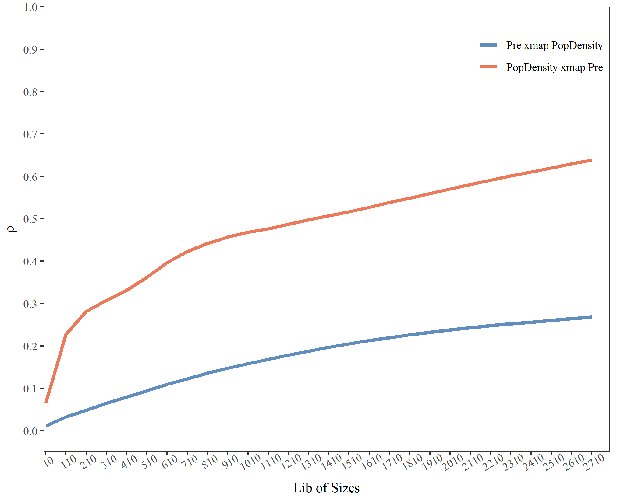
An example of spatial grid data
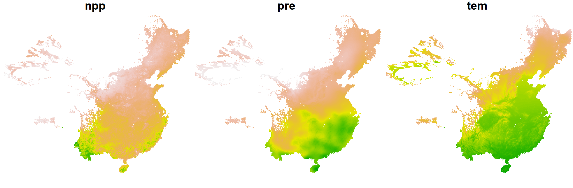
Load the spEDM package and its farmland NPP data:
library(spEDM)

npp = terra::rast(system.file("case/npp.tif", package = "spEDM"))
# To save the computation time, we will aggregate the data by 3 times
npp = terra::aggregate(npp, fact = 3, na.rm = TRUE)
npp
## class       : SpatRaster
## size        : 135, 161, 5  (nrow, ncol, nlyr)
## resolution  : 30000, 30000  (x, y)
## extent      : -2625763, 2204237, 1867078, 5917078  (xmin, xmax, ymin, ymax)
## coord. ref. : CGCS2000_Albers
## source(s)   : memory
## names       :      npp,        pre,      tem,      elev,         hfp
## min values  :   187.50,   390.3351, -47.8194, -110.1494,  0.04434316
## max values  : 15381.89, 23734.5330, 262.8576, 5217.6431, 42.68803711

# Inspect NA values
terra::global(npp,"isNA")
##       isNA
## npp  14815
## pre  14766
## tem  14766
## elev 14760
## hfp  14972
terra::ncell(npp)
## [1] 21735
nnamat = terra::as.matrix(npp[[1]], wide = TRUE)
nnaindice = which(!is.na(nnamat), arr.ind = TRUE)
dim(nnaindice)
## [1] 6920    2

# Select 1500 non-NA pixels to predict:
set.seed(2025)
indices = sample(nrow(nnaindice), size = 1500, replace = FALSE)
libindice = nnaindice[-indices,]
predindice = nnaindice[indices,]
Determining optimal embedding dimension:
spEDM::simplex(npp, "pre", "pre", E = 2:10, k = 12, lib = nnaindice, pred = predindice)
## The suggested E,k,tau for variable pre is 2, 12 and 1
spEDM::simplex(npp, "npp", "npp", E = 2:10, k = 12, lib = nnaindice, pred = predindice)
## The suggested E,k,tau for variable npp is 10, 12 and 1
Run GCCM:
startTime = Sys.time()
npp_res = spEDM::gccm(data = npp, cause = "pre", effect = "npp",
                      libsizes = matrix(rep(seq(10,130,20),2),ncol = 2),
                      E = c(2,10), k = 12, lib = nnaindice, pred = predindice,
                      progressbar = FALSE)
endTime = Sys.time()
print(difftime(endTime,startTime, units ="mins"))
## Time difference of 1.097801 mins
npp_res
##   libsizes  pre->npp  npp->pre
## 1       10 0.1235069 0.1061684
## 2       30 0.2629126 0.2340358
## 3       50 0.3780635 0.3031695
## 4       70 0.4980299 0.3450645
## 5       90 0.5954949 0.3434175
## 6      110 0.7297306 0.3453495
## 7      130 0.8272545 0.3677895
Visualize the result:
plot(npp_res,xlimits = c(5, 135),ylimits = c(0.05,1), draw_ci = TRUE) +
  ggplot2::theme(legend.justification = c(0.25,1))