geographical convergent cross mapping

Usage

# S4 method for class 'sf'
gccm(
  data,
  cause,
  effect,
  libsizes,
  E = c(3, 3),
  tau = 1,
  k = 4,
  theta = 1,
  algorithm = "simplex",
  pred = NULL,
  nb = NULL,
  threads = detectThreads(),
  bidirectional = TRUE,
  trend.rm = TRUE,
  progressbar = TRUE
)

# S4 method for class 'SpatRaster'
gccm(
  data,
  cause,
  effect,
  libsizes,
  E = c(3, 3),
  tau = 1,
  k = 4,
  theta = 1,
  algorithm = "simplex",
  pred = NULL,
  threads = detectThreads(),
  bidirectional = TRUE,
  trend.rm = TRUE,
  progressbar = TRUE
)

Arguments

data: The observation data.
cause: Name of causal variable.
effect: Name of effect variable.
libsizes: A vector of library sizes to use.
E: (optional) Dimensions of the embedding.
tau: (optional) Step of spatial lags.
k: (optional) Number of nearest neighbors to use for prediction.
theta: (optional) Weighting parameter for distances, useful when algorithm is smap.
algorithm: (optional) Algorithm used for prediction.
pred: pred (optional) Row numbers(vector) of lattice data or row-column numbers(matrix) of grid data used for predictions.
nb: (optional) The neighbours list.
threads: (optional) Number of threads.
bidirectional: (optional) whether to identify bidirectional causal associations.
trend.rm: (optional) Whether to remove the linear trend.
progressbar: (optional) whether to print the progress bar.

Value

A list.

xmap: cross mapping prediction results
varname: names of causal and effect variable
bidirectional: whether to identify bidirectional causal associations

Examples

columbus = sf::read_sf(system.file("shapes/columbus.gpkg", package="spData"))
# \donttest{
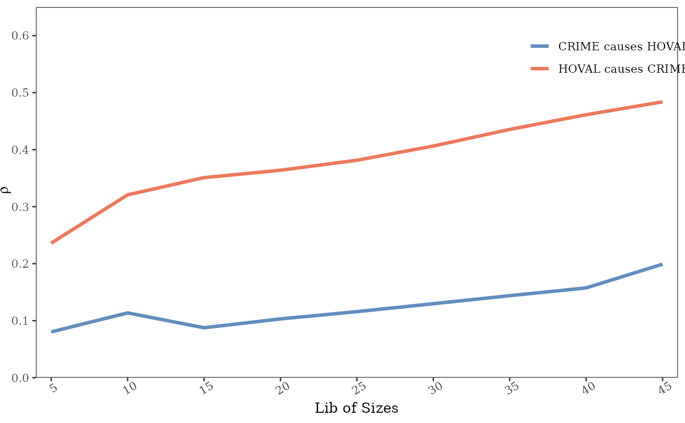
g = gccm(columbus,"HOVAL","CRIME",libsizes = seq(5,40,5),E = 6)
#> 
Computing: [========================================] 100% (done)                         
#> 
Computing: [========================================] 100% (done)                         
g
#>   libsizes HOVAL->CRIME CRIME->HOVAL
#> 1        5    0.1323440    0.2804058
#> 2       10    0.2440359    0.4006664
#> 3       15    0.2426027    0.4609814
#> 4       20    0.2195416    0.5019578
#> 5       25    0.2251323    0.5452084
#> 6       30    0.2448081    0.5847262
#> 7       35    0.2562830    0.6019328
#> 8       40    0.2749386    0.6217028
plot(g, ylimits = c(0,0.85))

# }