Spatial Logistic Map

Wenbo Lv

Last update: 2025-08-27
Last run: 2025-08-27

Methodological Background

The logistic map is one of the most fundamental nonlinear dynamical systems used to explore the transition from regularity to chaos. In its univariate temporal form, the logistic map is expressed as:

\[ x_{t+1} = r x_t (1 - x_t), \]

where \(x_t \in [0,1]\) is the state of the system at time \(t\), and \(r\) is a growth parameter. Despite its algebraic simplicity, the logistic map exhibits a rich spectrum of dynamical behaviors, including bifurcations, periodic orbits, and deterministic chaos, depending on the value of \(r\). Its sensitivity to initial conditions and nonlinear feedback makes it a canonical model for exploring complex temporal dynamics.

In multivariate extensions of the logistic map, such as coupled logistic systems, each variable evolves under its own logistic rule but is also influenced by the states of other variables. A common form is:

\[ x_{t+1}^{(i)} = r_i x_t^{(i)} \left(1 - x_t^{(i)} - \sum_{j \neq i} \beta_{ij} x_t^{(j)} \right), \]

where \(\beta_{ij}\) denotes the inhibitory (or facilitative) effect of variable \(j\) on variable \(i\). These multivariate systems allow the study of interaction-driven complexity, including predator-prey dynamics, interspecies competition, and coevolutionary processes.

This framework can be further extended to spatial domains to account for interactions among neighboring spatial units. The resulting system, known as the Spatial Logistic Map (SLM), distributes the logistic dynamics over a spatial lattice. In the simplest case, each location \(i\) on the lattice updates according to:

\[ x_{i}^{(t+1)} = 1 - \alpha x_i^{(t)} \cdot \frac{1}{k} \sum_{j \in \mathcal{N}(i)} x_j^{(t)}, \]

where \(\alpha\) controls the strength of nonlinearity and spatial coupling, \(\mathcal{N}(i)\) denotes the set of spatial neighbors (e.g., rook- or queen-connected units), and \(k = |\mathcal{N}(i)|\) is the number of neighbors. This form reflects a local averaging interaction: the future value of a unit depends on its current value and the average state of its neighbors.

Importantly, when extended to multivariate spatial settings, such as bivariate or trivariate spatial logistic maps, each spatial variable evolves not only through its own neighbors but also through inter-variable interactions. For example, in a bivariate spatial logistic map, the update rules may be written as:

• Local cross-variable interaction (default form):

\[ x_{i}^{(t+1)} = 1 - \alpha_1 x_i^{(t)} \left( \frac{1}{k} \sum_{j \in \mathcal{N}(i)} x_j^{(t)} - \beta_{21} y_i^{(t)} \right), \\ y_{i}^{(t+1)} = 1 - \alpha_2 y_i^{(t)} \left( \frac{1}{k} \sum_{j \in \mathcal{N}(i)} y_j^{(t)} - \beta_{12} x_i^{(t)} \right). \]

Here, the inhibitory (or facilitative) influence between variables is restricted to the same spatial location.

• Neighbor-averaged cross-variable interaction (extended form):

\[ x_{i}^{(t+1)} = 1 - \alpha_1 x_i^{(t)} \left( \frac{1}{k} \sum_{j \in \mathcal{N}(i)} x_j^{(t)} - \beta_{21} \frac{1}{k} \sum_{j \in \mathcal{N}(i)} y_j^{(t)} \right), \\ y_{i}^{(t+1)} = 1 - \alpha_2 y_i^{(t)} \left( \frac{1}{k} \sum_{j \in \mathcal{N}(i)} y_j^{(t)} - \beta_{12} \frac{1}{k} \sum_{j \in \mathcal{N}(i)} x_j^{(t)} \right). \]

In this alternative form, the inter-variable interactions are mediated through the neighbor-averaged states, allowing each variable to be influenced by the spatial context of the other.

Both formulations capture the combination of local spatial coupling and cross-variable inhibition, but they differ in whether the cross-variable effects are purely local or spatially contextualized. These distinctions lead to different spatiotemporal outcomes, including waves, kinks, frozen random states, and spatiotemporal chaos.

By performing statistical aggregation over the long-run time series values at each spatial unit, one can generate spatial cross-sectional data that reflect different causal scenarios.

Usage examples

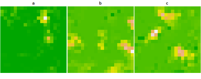
We first construct three simulated species density distributions by combining a Gaussian random field with a multivariate normal distribution.

sim_trispecies = \(nx,ny,seed = 123){
  grid = expand.grid(seq(0, 10, length.out = nx),
                     seq(0, 10, length.out = ny))
  cov.fun = \(d, range = 1.5, sill=1) sill * exp(-d/range)
  dist.mat = fields::rdist(grid)
  cov.mat = cov.fun(dist.mat, range=1.5, sill=1)
  set.seed(seed)
  res = replicate(3, {
    MASS::mvrnorm(1, rep(0, nrow(grid)), cov.mat) |>
      pmax(0) |>
      sdsfun::normalize_vector(0,1) |>
      matrix(nrow = nx, ncol = ny) |>
      terra::rast()
  }, simplify = FALSE)
  terra::rast(res)
}

species = sim_trispecies(20,20)
names(species) = letters[1:3]
species
## class       : SpatRaster 
## size        : 20, 20, 3  (nrow, ncol, nlyr)
## resolution  : 1, 1  (x, y)
## extent      : 0, 20, 0, 20  (xmin, xmax, ymin, ymax)
## coord. ref. :  
## source(s)   : memory
## names       : a, b, c 
## min values  : 0, 0, 0 
## max values  : 1, 1, 1

options(terra.pal = grDevices::terrain.colors(100,rev = T))
terra::plot(species, nc = 3,
            mar = rep(0.1,4),
            oma = rep(0.1,4),
            axes = FALSE,
            legend = FALSE)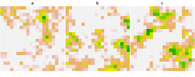

Figure 1. Simulated initial species density distributions for three species (a, b, and c).

We assume an underlying causal interaction structure among species, where species a influences b, and b in turn influences c (i.e., a → b → c). The intrinsic growth rates of species a, b, and c are uniformly assigned a value of 0.2. Species a exerts an effect of 1 on species b, and species b exerts an effect of 1 on species c. All other interspecific influence parameters are set to 0. This setup provides a controlled environment to test spatial causality detection methods under known dynamic interactions.

simv = spEDM::slm(species, x = "a", y = "b", z = "c", k = 4, step = 15, transient = 1, interact = "local",
                  alpha_x = 0.2, alpha_y = 0.2, alpha_z = 0.2,
                  beta_xy = 1, beta_xz = 0, beta_yx = 0, beta_yz = 1, beta_zx = 0, beta_zy = 0)

species_evolution = species
terra::values(species_evolution[["a"]]) = simv$x
terra::values(species_evolution[["b"]]) = simv$y
terra::values(species_evolution[["c"]]) = simv$z
species_evolution
## class       : SpatRaster 
## size        : 20, 20, 3  (nrow, ncol, nlyr)
## resolution  : 1, 1  (x, y)
## extent      : 0, 20, 0, 20  (xmin, xmax, ymin, ymax)
## coord. ref. :  
## source(s)   : memory
## names       :         a,         b,         c 
## min values  : 0.8553408, 0.9733337, 0.9886246 
## max values  : 0.8611597, 0.9803933, 1.0008822

terra::plot(species_evolution, nc = 3,
            mar = rep(0.1,4),
            oma = rep(0.1,4),
            axes = FALSE,
            legend = FALSE)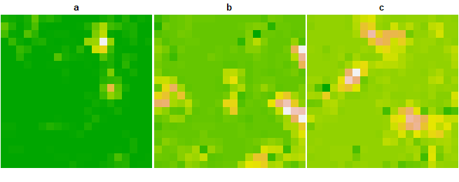

Figure 2. Species distributions following spatiotemporal interaction and evolution after 20 simulation steps with 4-neighbor interactions.

simv = spEDM::slm(species, x = "a", y = "b", z = "c", k = 4, step = 15, transient = 1, interact = "neighbors",
                  alpha_x = 0.2, alpha_y = 0.2, alpha_z = 0.2, beta_xy = 1, beta_xz = 0, beta_yx = 0, beta_yz = 1, beta_zx = 0, beta_zy = 0)

species_evolution = species
terra::values(species_evolution[["a"]]) = simv$x
terra::values(species_evolution[["b"]]) = simv$y
terra::values(species_evolution[["c"]]) = simv$z
species_evolution
## class       : SpatRaster 
## size        : 20, 20, 3  (nrow, ncol, nlyr)
## resolution  : 1, 1  (x, y)
## extent      : 0, 20, 0, 20  (xmin, xmax, ymin, ymax)
## coord. ref. :  
## source(s)   : memory
## names       :         a,         b,         c 
## min values  : 0.8553408, 0.9718102, 0.9887262 
## max values  : 0.8611597, 0.9803232, 0.9986816

terra::plot(species_evolution, nc = 3,
            mar = rep(0.1,4),
            oma = rep(0.1,4),
            axes = FALSE,
            legend = FALSE)

Figure 3. Species distributions after 20 simulation steps with 4-neighbor interactions and neighbor-averaged cross-variable dynamics.