Overview
The spEDM package is an open-source, computationally efficient toolkit designed to provide a unified API for Spatial Empirical Dynamic Modeling. It supports a suite of prediction-based causal inference algorithms, including spatial (granger) causality test, geographically convergent cross mapping, and geographical cross mapping cardinality.
To support both learning and practical application, spEDM offers four carefully curated spatial cross-sectional datasets, each paired with a detailed example showcasing the use of key algorithms in the package.
Installation
Install the stable version from CRAN with:
install.packages("spEDM", dep = TRUE)Alternatively, you can install the development version from R-universe with:
install.packages("spEDM",
                 repos = c("https://stscl.r-universe.dev",
                           "https://cloud.r-project.org"),
                 dep = TRUE)
Data
The spEDM package includes four illustrative datasets with well-known causation to demonstrate key functionalities:
Columbus, OH dataset — A classic spatial dataset widely used in spatial econometrics, included here for benchmarking and demonstration purposes. Data files:
columbus.gpkgPopulation density and its potential drivers in mainland China — A county-level dataset capturing population density alongside relevant socio-environmental drivers. Data files:
popd.csv,popd_nb.galSoil copper (Cu) contamination — A raster-based dataset representing soil Cu concentrations, with associated layers on nighttime light intensity and industrial density, useful for exploring the influence of human activities on environmental pollution. Data files:
cu.tifFarmland NPP and related variables — A raster dataset capturing net primary productivity (NPP) of farmland, key climatic variables, elevation, and human activity footprints across mainland China, suitable for analyzing the interactions between agricultural productivity, environmental conditions, and human activities. Data files:
npp.tif
These datasets can be loaded as shown below, including basic visualization for raster data:
Columbus OH spatial analysis dataset
library(spEDM)

columbus = sf::read_sf(system.file("case/columbus.gpkg", package="spEDM"))
columbus
## Simple feature collection with 49 features and 6 fields
## Geometry type: POLYGON
## Dimension:     XY
## Bounding box:  xmin: 5.874907 ymin: 10.78863 xmax: 11.28742 ymax: 14.74245
## Projected CRS: Undefined Cartesian SRS with unknown unit
## # A tibble: 49 × 7
##    hoval   inc  crime  open plumb discbd                                     geom
##    <dbl> <dbl>  <dbl> <dbl> <dbl>  <dbl>                                <POLYGON>
##  1  80.5 19.5  15.7   2.85  0.217   5.03 ((8.624129 14.23698, 8.5597 14.74245, 8…
##  2  44.6 21.2  18.8   5.30  0.321   4.27 ((8.25279 14.23694, 8.282758 14.22994, …
##  3  26.4 16.0  30.6   4.53  0.374   3.89 ((8.653305 14.00809, 8.81814 14.00205, …
##  4  33.2  4.48 32.4   0.394 1.19    3.7  ((8.459499 13.82035, 8.473408 13.83227,…
##  5  23.2 11.3  50.7   0.406 0.625   2.83 ((8.685274 13.63952, 8.677577 13.72221,…
##  6  28.8 16.0  26.1   0.563 0.254   3.78 ((9.401384 13.5504, 9.434411 13.69427, …
##  7  75    8.44  0.178 0     2.40    2.74 ((8.037741 13.60752, 8.062716 13.60452,…
##  8  37.1 11.3  38.4   3.48  2.74    2.89 ((8.247527 13.58651, 8.2795 13.5965, 8.…
##  9  52.6 17.6  30.5   0.527 0.891   3.17 ((9.333297 13.27242, 9.671007 13.27361,…
## 10  96.4 13.6  34.0   1.55  0.558   4.33 ((10.08251 13.03377, 10.0925 13.05275, …
## # ℹ 39 more rows
County-level population density in mainland China
library(spEDM)

popd_nb = spdep::read.gal(system.file("case/popd_nb.gal",package = "spEDM"))
## Warning in spdep::read.gal(system.file("case/popd_nb.gal", package = "spEDM")):
## neighbour object has 4 sub-graphs
popd_nb
## Neighbour list object:
## Number of regions: 2806
## Number of nonzero links: 15942
## Percentage nonzero weights: 0.2024732
## Average number of links: 5.681397
## 4 disjoint connected subgraphs

popd = readr::read_csv(system.file("case/popd.csv",package = "spEDM"))
## Rows: 2806 Columns: 7
## ── Column specification ─────────────────────────────────────────────────────────
## Delimiter: ","
## dbl (7): x, y, popd, elev, tem, pre, slope
##
## ℹ Use `spec()` to retrieve the full column specification for this data.
## ℹ Specify the column types or set `show_col_types = FALSE` to quiet this message.
popd
## # A tibble: 2,806 × 7
##        x     y  popd  elev   tem   pre slope
##    <dbl> <dbl> <dbl> <dbl> <dbl> <dbl> <dbl>
##  1  117.  30.5  780.     8  17.4 1528. 0.452
##  2  117.  30.6  395.    48  17.2 1487. 0.842
##  3  117.  30.8  261.    49  16.0 1456. 3.56
##  4  116.  30.1  258.    23  17.4 1555. 0.932
##  5  116.  30.5  211.   101  16.3 1494. 3.34
##  6  117.  31.0  386.    10  16.6 1382. 1.65
##  7  117.  30.2  350.    23  17.5 1569. 0.346
##  8  117.  30.7  470.    22  17.1 1493. 1.88
##  9  117.  30.6 1226.    11  17.4 1526. 0.208
## 10  116.  30.9  137.   598  13.9 1458. 5.92
## # ℹ 2,796 more rows

popd_sf = sf::st_as_sf(popd, coords = c("x","y"), crs = 4326)
popd_sf
## Simple feature collection with 2806 features and 5 fields
## Geometry type: POINT
## Dimension:     XY
## Bounding box:  xmin: 74.9055 ymin: 18.2698 xmax: 134.269 ymax: 52.9346
## Geodetic CRS:  WGS 84
## # A tibble: 2,806 × 6
##     popd  elev   tem   pre slope          geometry
##  * <dbl> <dbl> <dbl> <dbl> <dbl>       <POINT [°]>
##  1  780.     8  17.4 1528. 0.452 (116.912 30.4879)
##  2  395.    48  17.2 1487. 0.842 (116.755 30.5877)
##  3  261.    49  16.0 1456. 3.56  (116.541 30.7548)
##  4  258.    23  17.4 1555. 0.932  (116.241 30.104)
##  5  211.   101  16.3 1494. 3.34   (116.173 30.495)
##  6  386.    10  16.6 1382. 1.65  (116.935 30.9839)
##  7  350.    23  17.5 1569. 0.346 (116.677 30.2412)
##  8  470.    22  17.1 1493. 1.88  (117.066 30.6514)
##  9 1226.    11  17.4 1526. 0.208 (117.171 30.5558)
## 10  137.   598  13.9 1458. 5.92  (116.208 30.8983)
## # ℹ 2,796 more rows
Soil Cu heavy metal contamination
library(spEDM)

cu = terra::rast(system.file("case/cu.tif", package="spEDM"))
cu
## class       : SpatRaster
## dimensions  : 131, 125, 3  (nrow, ncol, nlyr)
## resolution  : 5000, 5000  (x, y)
## extent      : 360000, 985000, 1555000, 2210000  (xmin, xmax, ymin, ymax)
## coord. ref. : North_American_1983_Albers
## source      : cu.tif
## names       :         cu, industry, ntl
## min values  :   1.201607,    0.000,   0
## max values  : 319.599274,    0.615,  63

options(terra.pal = grDevices::terrain.colors(100,rev = T))
terra::plot(cu, nc = 3,
            mar = rep(0.1,4),
            oma = rep(0.1,4),
            axes = FALSE,
            legend = FALSE)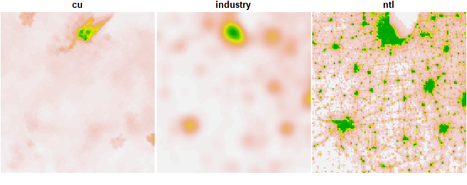
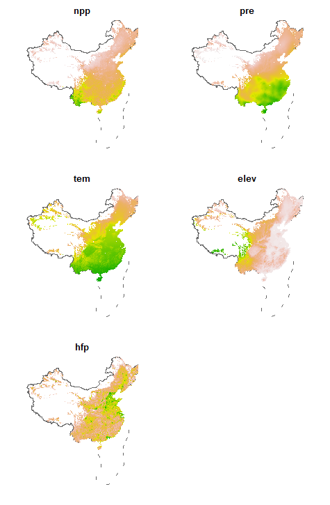
Farmland NPP and related variables in mainland China
library(spEDM)
npp = terra::rast(system.file("case/npp.tif", package = "spEDM"))
npp
## class       : SpatRaster
## dimensions  : 404, 483, 5  (nrow, ncol, nlyr)
## resolution  : 10000, 10000  (x, y)
## extent      : -2625763, 2204237, 1877078, 5917078  (xmin, xmax, ymin, ymax)
## coord. ref. : CGCS2000_Albers
## source      : npp.tif
## names       :      npp,        pre,      tem,      elev,         hfp
## min values  :   164.00,   384.3409, -47.8194, -122.2004,  0.03390418
## max values  : 16606.33, 23878.3555, 263.6938, 5350.4902, 44.90312195

# directly visualize the raster layer
options(terra.pal = grDevices::terrain.colors(100,rev = T))
terra::plot(npp, nc = 2,
            axes = FALSE,
            legend = FALSE)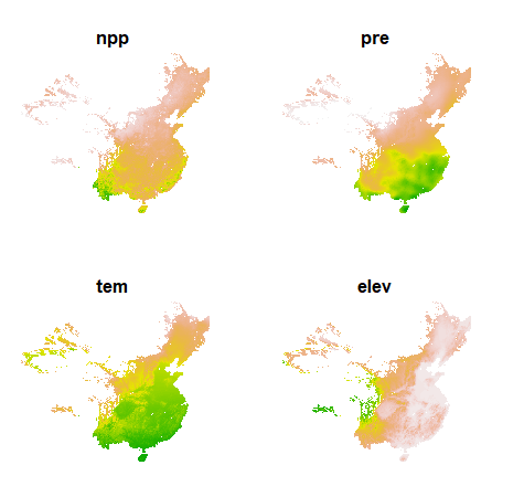
# add China's land borders and the ten-dash line in the South China Sea

# install.packages("geocn",
#                  repos = c("https://stscl.r-universe.dev",
#                            "https://cloud.r-project.org"),
#                  dep = TRUE)

cn_border = geocn::load_cn_border() |>
  terra::vect() |>
  terra::project(terra::crs(npp))

par(mfrow = c(3, 2))
for (i in 1:terra::nlyr(npp)) {
  terra::plot(cn_border, lwd = 1.5, main = names(npp)[i],
              col = "grey40", axes = FALSE)
  terra::plot(npp[[i]], axes = FALSE,
              legend = FALSE, add = TRUE)
}
Usage
Users can refer to several additional vignettes for more detailed examples of using spEDM, namely:
| Model | Vignette |
|---|---|
| State Space Reconstruction | SSR |
| Geographical Convergent Cross Mapping | GCCM |
| Geographical Cross Mapping Cardinality | GCMC |
| Spatial Causality Test | SCT |
In addition to the spatial extensions provided by spEDM, several other R packages support Empirical Dynamic Modeling (EDM) for time series data:
- rEDM: A foundational EDM package implementing simplex projection, S-map, and convergent cross mapping (CCM), widely used for analyzing nonlinear time series dynamics.
- multispatialCCM: Implements CCM for collections of short time series using bootstrapping, enabling causal inference across replicated or multi-site time series.
- fastEDM: A high-performance EDM package with a multi-threaded C++ backend. It supports large-scale time series analysis, handles panel data, and provides robust options for dealing with missing values using delay-tolerant algorithms or data exclusion.
References
Takens, F. (1981). Detecting strange attractors in turbulence. Dynamical Systems and Turbulence, Warwick 1980, 366–381. https://doi.org/10.1007/bfb0091924
Mañé, R. (1981). On the dimension of the compact invariant sets of certain non-linear maps. Dynamical Systems and Turbulence, Warwick 1980, 230–242. https://doi.org/10.1007/bfb0091916
Herrera, M., Mur, J., & Ruiz, M. (2016). Detecting causal relationships between spatial processes. Papers in Regional Science, 95(3), 577–595. https://doi.org/10.1111/pirs.12144
Gao, B., Yang, J., Chen, Z., Sugihara, G., Li, M., Stein, A., Kwan, M.-P., & Wang, J. (2023). Causal inference from cross-sectional earth system data with geographical convergent cross mapping. Nature Communications, 14(1). https://doi.org/10.1038/s41467-023-41619-6