Geographical Pattern Causality
Wenbo Lv
Last
update: 2025-11-25
Last run: 2025-11-30
Source: Last run: 2025-11-30
vignettes/GPC.Rmd
GPC.RmdMethodological Background
Geographical Pattern Causality (GPC) infers causal relations from spatial cross-sectional data by reconstructing a symbolic approximation of the underlying spatial dynamical system.
Let \(x(s)\) and \(y(s)\) denote two spatial cross-sections over locations \(s \in \mathcal{S}\).
(1) Spatial Embedding
For each location \(s_i\), GPC constructs an embedding vector
\[ \mathbf{E}_{x(s_i)} = \big( x(s_{i}^{(1)}), x(s_{i}^{(2)}), \dots, x(s_{i}^{(E\tau)}) \big), \]
where \(s_{i}^{(k)}\) denotes the \(k\)-th spatially lagged value of the spatial unit \(s_i\), determined by embedding dimension \(E\) and lag \(\tau\). This yields two reconstructed state spaces \(\mathcal{M}_x, \mathcal{M}_y \subset \mathbb{R}^E\).
(2) Symbolic Pattern Extraction
Local geometric transitions in each manifold are mapped to symbols
\[ \sigma_x(s_i),; \sigma_y(s_i) \in \mathcal{A}, \]
encoding increasing, decreasing, or non-changing modes. These symbolic trajectories summarize local pattern evolution.
(3) Cross-Pattern Mapping
Causality from \(x \to y\) is assessed by predicting:
\[ \hat{\sigma}_y(s_i) = F\big( \sigma_x(s_j): s_j \in \mathcal{N}_k(s_i) \big), \]
where \(\mathcal{N}_k\) denotes the set of \(k\) nearest neighbors in \(\mathcal{M}_x\). The agreement structure between \(\hat{\sigma}_y(s_i)\) and \(\sigma_y(s_i)\) determines the causal mode:
- Positive: \(\hat{\sigma}_y = \sigma_y\)
- Negative: \(\hat{\sigma}_y = -\sigma_y\)
- Dark: neither agreement nor opposition
(4) Causal Strength
The global causal strength is the normalized consistency of symbol matches:
\[ C_{x \to y} = \frac{1}{|\mathcal{S}|} \sum_{s_i \in \mathcal{S}} \mathbb{I}\big[ \hat{\sigma}_y(s_i) \bowtie \sigma_y(s_i) \big], \]
where \(\bowtie\) encodes positive, negative, or dark matching rules.
Usage examples
An example of spatial lattice data
Load the spEDM package and its columbus spatial analysis
data:
library(spEDM)

columbus = sf::read_sf(system.file("case/columbus.gpkg", package="spEDM"))
columbus
## Simple feature collection with 49 features and 6 fields
## Geometry type: POLYGON
## Dimension:     XY
## Bounding box:  xmin: 5.874907 ymin: 10.78863 xmax: 11.28742 ymax: 14.74245
## Projected CRS: Undefined Cartesian SRS with unknown unit
## # A tibble: 49 × 7
##    hoval   inc  crime  open plumb discbd                                    geom
##    <dbl> <dbl>  <dbl> <dbl> <dbl>  <dbl>                               <POLYGON>
##  1  80.5 19.5  15.7   2.85  0.217   5.03 ((8.624129 14.23698, 8.5597 14.74245, …
##  2  44.6 21.2  18.8   5.30  0.321   4.27 ((8.25279 14.23694, 8.282758 14.22994,…
##  3  26.4 16.0  30.6   4.53  0.374   3.89 ((8.653305 14.00809, 8.81814 14.00205,…
##  4  33.2  4.48 32.4   0.394 1.19    3.7  ((8.459499 13.82035, 8.473408 13.83227…
##  5  23.2 11.3  50.7   0.406 0.625   2.83 ((8.685274 13.63952, 8.677577 13.72221…
##  6  28.8 16.0  26.1   0.563 0.254   3.78 ((9.401384 13.5504, 9.434411 13.69427,…
##  7  75    8.44  0.178 0     2.40    2.74 ((8.037741 13.60752, 8.062716 13.60452…
##  8  37.1 11.3  38.4   3.48  2.74    2.89 ((8.247527 13.58651, 8.2795 13.5965, 8…
##  9  52.6 17.6  30.5   0.527 0.891   3.17 ((9.333297 13.27242, 9.671007 13.27361…
## 10  96.4 13.6  34.0   1.55  0.558   4.33 ((10.08251 13.03377, 10.0925 13.05275,…
## # ℹ 39 more rows
The false nearest neighbours (FNN) method helps identify the appropriate minimal embedding dimension for reconstructing the state space of a time series or spatial cross-sectional data.
spEDM::fnn(columbus, "crime", E = 1:10, eps = stats::sd(columbus$crime))
##        E:1        E:2        E:3        E:4        E:5        E:6        E:7
## 0.59183673 0.04081633 0.04081633 0.10204082 0.00000000 0.00000000 0.00000000
##        E:8
## 0.00000000
The false nearest neighbours (FNN) ratio decreased to approximately 0.001 when the embedding dimension E reached 7, and remained relatively stable thereafter. Therefore, we adopted \(E = 7\) as the minimal embedding dimension for subsequent parameter search.
Then, search optimal parameters:
# determine the type of causality using correlation
stats::cor.test(columbus$hoval,columbus$crime)
##
##  Pearson's product-moment correlation
##
## data:  columbus$hoval and columbus$crime
## t = -4.8117, df = 47, p-value = 1.585e-05
## alternative hypothesis: true correlation is not equal to 0
## 95 percent confidence interval:
##  -0.7366777 -0.3497978
## sample estimates:
##        cor
## -0.5744867

# since the correlation is -0.574, negative causality is selected as the metric to maximize in the optimal parameter search
spEDM::pc(columbus, "hoval", "crime", E = 5:6, k = 7:10, tau = 1, maximize = "negative")
## The suggested E,k,tau for variable crime is 6, 9 and 1
Run geographical pattern causality analysis
spEDM::gpc(columbus, "hoval", "crime", E = 6, k = 9)
## --------------------------------
## ***pattern causality analysis***
## --------------------------------
##       type  strength      direction
## 1 positive       NaN hoval -> crime
## 2 negative 0.1340069 hoval -> crime
## 3     dark 0.1043991 hoval -> crime
## 4 positive       NaN crime -> hoval
## 5 negative 0.6251773 crime -> hoval
## 6     dark 0.1468990 crime -> hoval
Convergence diagnostics
crime_convergence = spEDM::gpc(columbus, "hoval", "crime",
                               libsizes = seq(5, 45, by = 5),
                               E = 6, k = 9, progressbar = FALSE)
crime_convergence
## --------------------------------
## ***pattern causality analysis***
## --------------------------------
##    libsizes     type        mean        q05        q50        q95
## 1        10 positive 0.000000000 0.00000000 0.00000000 0.00000000
## 2        15 positive 0.000000000 0.00000000 0.00000000 0.00000000
## 3        20 positive 0.000000000 0.00000000 0.00000000 0.00000000
## 4        25 positive 0.000000000 0.00000000 0.00000000 0.00000000
## 5        30 positive 0.000000000 0.00000000 0.00000000 0.00000000
## 6        35 positive 0.000000000 0.00000000 0.00000000 0.00000000
## 7        40 positive 0.000000000 0.00000000 0.00000000 0.00000000
## 8        45 positive 0.000000000 0.00000000 0.00000000 0.00000000
## 9        10 negative 0.070625218 0.00000000 0.00000000 0.30659823
## 10       15 negative 0.115077546 0.00000000 0.10275505 0.30880682
## 11       20 negative 0.108616161 0.00000000 0.10662265 0.24102060
## 12       25 negative 0.121201874 0.04592266 0.11589173 0.21679072
## 13       30 negative 0.131173338 0.04875268 0.13260719 0.23211138
## 14       35 negative 0.135053399 0.05939354 0.12811574 0.23473999
## 15       40 negative 0.143462998 0.06274451 0.13875013 0.22583851
## 16       45 negative 0.132237392 0.05154815 0.13400692 0.20321523
## 17       10     dark 0.017014322 0.00000000 0.01608876 0.04951971
## 18       15     dark 0.022611842 0.00000000 0.01861307 0.05769873
## 19       20     dark 0.021763180 0.00000000 0.02173713 0.04624619
## 20       25     dark 0.022012245 0.00000000 0.01813809 0.05928351
## 21       30     dark 0.042402814 0.00000000 0.04362907 0.08131942
## 22       35     dark 0.051311033 0.01622624 0.04623515 0.10253654
## 23       40     dark 0.071720825 0.03282035 0.06830303 0.11263398
## 24       45     dark 0.090931207 0.05514622 0.09094789 0.12987726
## 25       10 positive 0.000000000 0.00000000 0.00000000 0.00000000
## 26       15 positive 0.000000000 0.00000000 0.00000000 0.00000000
## 27       20 positive 0.000000000 0.00000000 0.00000000 0.00000000
## 28       25 positive 0.000000000 0.00000000 0.00000000 0.00000000
## 29       30 positive 0.000000000 0.00000000 0.00000000 0.00000000
## 30       35 positive 0.000000000 0.00000000 0.00000000 0.00000000
## 31       40 positive 0.000000000 0.00000000 0.00000000 0.00000000
## 32       45 positive 0.000000000 0.00000000 0.00000000 0.00000000
## 33       10 negative 0.008533609 0.00000000 0.00000000 0.00000000
## 34       15 negative 0.000000000 0.00000000 0.00000000 0.00000000
## 35       20 negative 0.005673075 0.00000000 0.00000000 0.00000000
## 36       25 negative 0.007707627 0.00000000 0.00000000 0.00000000
## 37       30 negative 0.056205723 0.00000000 0.00000000 0.51354762
## 38       35 negative 0.167157122 0.00000000 0.10376552 0.62340830
## 39       40 negative 0.337778689 0.00000000 0.30424357 0.62517731
## 40       45 negative 0.571883820 0.08335697 0.62517731 0.62517731
## 41       10     dark 0.074196224 0.03913357 0.07618520 0.10862499
## 42       15     dark 0.083670433 0.04180185 0.08637332 0.11457037
## 43       20     dark 0.098846255 0.06356219 0.09795915 0.14037150
## 44       25     dark 0.103796838 0.07022535 0.10459567 0.13903714
## 45       30     dark 0.112353198 0.08234950 0.11259679 0.15063914
## 46       35     dark 0.118136046 0.08068679 0.11467853 0.15527543
## 47       40     dark 0.131994205 0.08956014 0.13381611 0.16799219
## 48       45     dark 0.142222189 0.10399541 0.14525108 0.17518310
##         direction
## 1  hoval -> crime
## 2  hoval -> crime
## 3  hoval -> crime
## 4  hoval -> crime
## 5  hoval -> crime
## 6  hoval -> crime
## 7  hoval -> crime
## 8  hoval -> crime
## 9  hoval -> crime
## 10 hoval -> crime
## 11 hoval -> crime
## 12 hoval -> crime
## 13 hoval -> crime
## 14 hoval -> crime
## 15 hoval -> crime
## 16 hoval -> crime
## 17 hoval -> crime
## 18 hoval -> crime
## 19 hoval -> crime
## 20 hoval -> crime
## 21 hoval -> crime
## 22 hoval -> crime
## 23 hoval -> crime
## 24 hoval -> crime
## 25 crime -> hoval
## 26 crime -> hoval
## 27 crime -> hoval
## 28 crime -> hoval
## 29 crime -> hoval
## 30 crime -> hoval
## 31 crime -> hoval
## 32 crime -> hoval
## 33 crime -> hoval
## 34 crime -> hoval
## 35 crime -> hoval
## 36 crime -> hoval
## 37 crime -> hoval
## 38 crime -> hoval
## 39 crime -> hoval
## 40 crime -> hoval
## 41 crime -> hoval
## 42 crime -> hoval
## 43 crime -> hoval
## 44 crime -> hoval
## 45 crime -> hoval
## 46 crime -> hoval
## 47 crime -> hoval
## 48 crime -> hoval
plot(crime_convergence, ylimits = c(-0.01,1),
     xlimits = c(9,46), xbreaks = seq(10, 45, 10))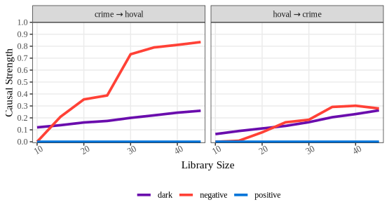
An example of spatial grid data
Load the spEDM package and its farmland NPP data:
library(spEDM)

npp = terra::rast(system.file("case/npp.tif", package = "spEDM"))
# To save the computation time, we will aggregate the data by 3 times
npp = terra::aggregate(npp, fact = 3, na.rm = TRUE)
npp
## class       : SpatRaster
## size        : 135, 161, 5  (nrow, ncol, nlyr)
## resolution  : 30000, 30000  (x, y)
## extent      : -2625763, 2204237, 1867078, 5917078  (xmin, xmax, ymin, ymax)
## coord. ref. : CGCS2000_Albers
## source(s)   : memory
## names       :      npp,        pre,      tem,      elev,         hfp
## min values  :   187.50,   390.3351, -47.8194, -110.1494,  0.04434316
## max values  : 15381.89, 23734.5330, 262.8576, 5217.6431, 42.68803711

# Check the validated cell number
nnamat = terra::as.matrix(npp[[1]], wide = TRUE)
nnaindice = which(!is.na(nnamat), arr.ind = TRUE)
dim(nnaindice)
## [1] 6920    2
Determining minimal embedding dimension:
spEDM::fnn(npp, "npp", E = 1:15,
           eps = stats::sd(terra::values(npp[["npp"]]),na.rm = TRUE))
##          E:1          E:2          E:3          E:4          E:5          E:6
## 0.9813070569 0.5309427415 0.1322254335 0.0167630058 0.0017341040 0.0000000000
##          E:7          E:8          E:9         E:10         E:11         E:12
## 0.0001445087 0.0000000000 0.0000000000 0.0000000000 0.0002890173 0.0000000000
##         E:13         E:14
## 0.0001445087 0.0001445087
At \(E = 6\), the false nearest neighbor ratio stabilizes approximately at 0.0001 and remains constant thereafter. Therefore, \(E = 6\) is selected as minimal embedding dimension for the subsequent GPC analysis.
Then, search optimal parameters:
stats::cor.test(~ pre + npp,
                data = terra::values(npp[[c("pre","npp")]],
                                      datafame = TRUE, na.rm = TRUE))
##
##  Pearson's product-moment correlation
##
## data:  pre and npp
## t = 108.74, df = 6912, p-value < 2.2e-16
## alternative hypothesis: true correlation is not equal to 0
## 95 percent confidence interval:
##  0.7855441 0.8029426
## sample estimates:
##       cor
## 0.7944062


g1 = spEDM::pc(npp, "npp", "pre", E = 6:10, k = 12, tau = 1:5, maximize = "positive")
g1
## The suggested E,k,tau for variable pre is 8, 12 and 5
Run geographical pattern causality analysis
spEDM::gpc(npp, "pre", "npp", E = 8, k = 12, tau = 5)
## --------------------------------
## ***pattern causality analysis***
## --------------------------------
##       type  strength  direction
## 1 positive 0.5348284 pre -> npp
## 2 negative       NaN pre -> npp
## 3     dark 0.4184010 pre -> npp
## 4 positive 0.4346310 npp -> pre
## 5 negative 0.0000000 npp -> pre
## 6     dark 0.3810809 npp -> pre
Convergence diagnostics
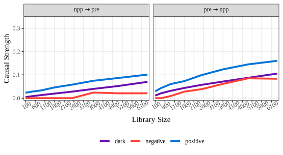
npp_convergence = spEDM::gpc(npp, "pre", "npp",
                             libsizes = matrix(rep(seq(10,80,10),2),ncol = 2),
                             E = 8, k = 12, tau = 5, progressbar = FALSE)
npp_convergence
## --------------------------------
## ***pattern causality analysis***
## --------------------------------
##    libsizes     type       mean        q05        q50        q95  direction
## 1       100 positive 0.13329950 0.07407592 0.12538196 0.21019892 pre -> npp
## 2       400 positive 0.18100175 0.14249619 0.18018497 0.22147429 pre -> npp
## 3       900 positive 0.25003464 0.21385822 0.24754501 0.29748254 pre -> npp
## 4      1600 positive 0.30971383 0.26851762 0.30981312 0.34501340 pre -> npp
## 5      2500 positive 0.37591136 0.34370484 0.37799443 0.40938124 pre -> npp
## 6      3600 positive 0.42811423 0.39096905 0.43029973 0.46082807 pre -> npp
## 7      4900 positive 0.46727140 0.43908847 0.46526482 0.49780759 pre -> npp
## 8      6400 positive 0.50712681 0.48845730 0.50607359 0.52917024 pre -> npp
## 9       100 negative 0.00000000 0.00000000 0.00000000 0.00000000 pre -> npp
## 10      400 negative 0.00000000 0.00000000 0.00000000 0.00000000 pre -> npp
## 11      900 negative 0.00000000 0.00000000 0.00000000 0.00000000 pre -> npp
## 12     1600 negative 0.00000000 0.00000000 0.00000000 0.00000000 pre -> npp
## 13     2500 negative 0.00000000 0.00000000 0.00000000 0.00000000 pre -> npp
## 14     3600 negative 0.00000000 0.00000000 0.00000000 0.00000000 pre -> npp
## 15     4900 negative 0.00000000 0.00000000 0.00000000 0.00000000 pre -> npp
## 16     6400 negative 0.00000000 0.00000000 0.00000000 0.00000000 pre -> npp
## 17      100     dark 0.06333096 0.04886528 0.06183032 0.08358828 pre -> npp
## 18      400     dark 0.11278520 0.10155495 0.11232502 0.12549444 pre -> npp
## 19      900     dark 0.17254903 0.16158658 0.17258621 0.18589246 pre -> npp
## 20     1600     dark 0.23544491 0.22435755 0.23518092 0.24744847 pre -> npp
## 21     2500     dark 0.29216320 0.28271925 0.29193486 0.30170269 pre -> npp
## 22     3600     dark 0.33692868 0.32827102 0.33645457 0.34721452 pre -> npp
## 23     4900     dark 0.37562510 0.36731091 0.37582609 0.38212762 pre -> npp
## 24     6400     dark 0.40905193 0.40228743 0.40879652 0.41570044 pre -> npp
## 25      100 positive 0.08370604 0.04391305 0.07934454 0.14943187 npp -> pre
## 26      400 positive 0.11837244 0.08625077 0.11817574 0.15751796 npp -> pre
## 27      900 positive 0.18424920 0.15435809 0.18403265 0.21228492 npp -> pre
## 28     1600 positive 0.26954887 0.23293732 0.26820265 0.31161775 npp -> pre
## 29     2500 positive 0.33977236 0.29821853 0.34026886 0.38175475 npp -> pre
## 30     3600 positive 0.38400895 0.35424047 0.38219004 0.42224626 npp -> pre
## 31     4900 positive 0.41104801 0.38079297 0.41126235 0.43664446 npp -> pre
## 32     6400 positive 0.42379598 0.40593770 0.42254648 0.44334792 npp -> pre
## 33      100 negative 0.00000000 0.00000000 0.00000000 0.00000000 npp -> pre
## 34      400 negative 0.00000000 0.00000000 0.00000000 0.00000000 npp -> pre
## 35      900 negative 0.00000000 0.00000000 0.00000000 0.00000000 npp -> pre
## 36     1600 negative 0.00000000 0.00000000 0.00000000 0.00000000 npp -> pre
## 37     2500 negative 0.00000000 0.00000000 0.00000000 0.00000000 npp -> pre
## 38     3600 negative 0.00000000 0.00000000 0.00000000 0.00000000 npp -> pre
## 39     4900 negative 0.00000000 0.00000000 0.00000000 0.00000000 npp -> pre
## 40     6400 negative 0.00000000 0.00000000 0.00000000 0.00000000 npp -> pre
## 41      100     dark 0.02942263 0.02228002 0.02919551 0.03682652 npp -> pre
## 42      400     dark 0.06566183 0.05533017 0.06567401 0.07682947 npp -> pre
## 43      900     dark 0.11924707 0.10860295 0.11937259 0.13028348 npp -> pre
## 44     1600     dark 0.18077129 0.17055326 0.18083090 0.19054978 npp -> pre
## 45     2500     dark 0.23789787 0.22516765 0.23808200 0.24874971 npp -> pre
## 46     3600     dark 0.28437360 0.27353890 0.28469842 0.29349259 npp -> pre
## 47     4900     dark 0.32567219 0.31519618 0.32666764 0.33424028 npp -> pre
## 48     6400     dark 0.36628717 0.36014813 0.36603708 0.37331526 npp -> pre
plot(npp_convergence, ylimits = c(-0.01,0.65),
     xlimits = c(0,6500), xbreaks = seq(100, 6400, 500))