Spatially Convergent Partial Cross Mapping
Wenbo Lyu
Last
update: 2026-02-15
Last run: 2026-04-05
Source: Last run: 2026-04-05
vignettes/main6_scpcm.Rmd
main6_scpcm.RmdModel principles
The methodological details are pending peer review and will be made available thereafter.
Usage examples
Example of spatial vector data
Load the spEDM package and columbus OH spatial analysis
dataset:
if (!requireNamespace("spEDM")) install.packages("spEDM")
## Loading required namespace: spEDM

columbus = sf::read_sf(system.file("case/columbus.gpkg", package="spEDM"))
columbus
## Simple feature collection with 49 features and 6 fields
## Geometry type: POLYGON
## Dimension:     XY
## Bounding box:  xmin: 5.874907 ymin: 10.78863 xmax: 11.28742 ymax: 14.74245
## Projected CRS: Undefined Cartesian SRS with unknown unit
## # A tibble: 49 × 7
##    hoval   inc  crime  open plumb discbd                                                  geom
##    <dbl> <dbl>  <dbl> <dbl> <dbl>  <dbl>                                             <POLYGON>
##  1  80.5 19.5  15.7   2.85  0.217   5.03 ((8.624129 14.23698, 8.5597 14.74245, 8.809452 14.73…
##  2  44.6 21.2  18.8   5.30  0.321   4.27 ((8.25279 14.23694, 8.282758 14.22994, 8.330711 14.2…
##  3  26.4 16.0  30.6   4.53  0.374   3.89 ((8.653305 14.00809, 8.81814 14.00205, 9.008951 13.9…
##  4  33.2  4.48 32.4   0.394 1.19    3.7  ((8.459499 13.82035, 8.473408 13.83227, 8.502935 13.…
##  5  23.2 11.3  50.7   0.406 0.625   2.83 ((8.685274 13.63952, 8.677577 13.72221, 8.90994 13.7…
##  6  28.8 16.0  26.1   0.563 0.254   3.78 ((9.401384 13.5504, 9.434411 13.69427, 9.605247 13.6…
##  7  75    8.44  0.178 0     2.40    2.74 ((8.037741 13.60752, 8.062716 13.60452, 8.072695 13.…
##  8  37.1 11.3  38.4   3.48  2.74    2.89 ((8.247527 13.58651, 8.2795 13.5965, 8.294443 13.604…
##  9  52.6 17.6  30.5   0.527 0.891   3.17 ((9.333297 13.27242, 9.671007 13.27361, 9.67701 13.2…
## 10  96.4 13.6  34.0   1.55  0.558   4.33 ((10.08251 13.03377, 10.0925 13.05275, 10.12649 13.0…
## # ℹ 39 more rows
We demonstrate how spatial vector data can be used in SCPCM analysis through a causal example examining the influences of the level of burglary incidents in a neighbourhood on house values, with neighbourhood household income included as a conditioning variable.
Determine minimum embedding dimensions:
spEDM::fnn(columbus,"crime",E = 1:10)
## [spEDM] Output 'E:i' corresponds to the i-th valid embedding dimension.
## [spEDM] Input E values exceeding max embeddable dimension were truncated.
## [spEDM] Please map output indices to original E inputs before interpretation.
##        E:1        E:2        E:3        E:4        E:5        E:6        E:7        E:8
## 0.79591837 0.53061224 0.63265306 0.51020408 0.12244898 0.04081633 0.00000000 0.00000000
spEDM::fnn(columbus,"hoval",E = 1:10)
## [spEDM] Output 'E:i' corresponds to the i-th valid embedding dimension.
## [spEDM] Input E values exceeding max embeddable dimension were truncated.
## [spEDM] Please map output indices to original E inputs before interpretation.
##        E:1        E:2        E:3        E:4        E:5        E:6        E:7        E:8
## 0.85714286 0.77551020 0.51020408 0.61224490 0.22448980 0.08163265 0.00000000 0.00000000
spEDM::fnn(columbus,"inc",E = 1:10)
## [spEDM] Output 'E:i' corresponds to the i-th valid embedding dimension.
## [spEDM] Input E values exceeding max embeddable dimension were truncated.
## [spEDM] Please map output indices to original E inputs before interpretation.
##        E:1        E:2        E:3        E:4        E:5        E:6        E:7        E:8
## 0.73469388 0.24489796 0.30612245 0.38775510 0.24489796 0.04081633 0.00000000 0.00000000
Self prediction for parameter turning:
spEDM::simplex(columbus,"crime","crime",E = 7:10,k=12)
## The suggested E,k,tau for variable crime is 8, 12 and 1
spEDM::simplex(columbus,"hoval","hoval",E = 7:10,k=12)
## The suggested E,k,tau for variable hoval is 7, 12 and 1
spEDM::simplex(columbus,"inc","inc",E = 7:10,k=12)
## The suggested E,k,tau for variable inc is 8, 12 and 1
Conduct SCPCM:
crime_hoval = spEDM::scpcm(data = columbus,
cause = "crime",
effect = "hoval",
conds = "inc",
libsizes = seq(5, 45, by = 5),
E = c(8,7,8),
k = 12,
progressbar = FALSE)
crime_hoval
## --------------------------------------
## ***partial cross mapping prediction***
## --------------------------------------
## libsizes crime->hoval hoval->crime
## 1 5 0.08948688 0.022401607
## 2 10 0.14511673 0.062986079
## 3 15 0.16849249 0.080653365
## 4 20 0.20940427 0.040974217
## 5 25 0.23160147 0.026613757
## 6 30 0.24709326 0.001942294
## 7 35 0.29707812 -0.014879976
## 8 40 0.33591810 -0.028758126
## 9 45 0.36337200 -0.040204136
##
## ------------------------------
## ***cross mapping prediction***
## ------------------------------
## libsizes crime->hoval hoval->crime
## 1 5 0.2224861 0.1378071
## 2 10 0.3023880 0.1880328
## 3 15 0.4005255 0.2085278
## 4 20 0.4681692 0.2203727
## 5 25 0.5098130 0.2293076
## 6 30 0.5467173 0.2326005
## 7 35 0.5732757 0.2331852
## 8 40 0.5822545 0.2361204
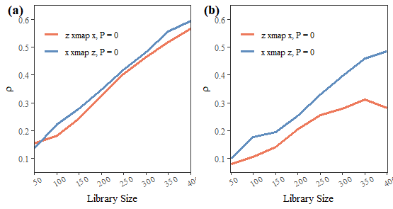
## 9 45 0.5883504 0.2364234Visualize the result:
if (!requireNamespace("cowplot")) install.packages("cowplot")
## Loading required namespace: cowplot

fig1a = plot(crime_hoval,partial = FALSE,ylimits = c(0.1,0.75))
fig1b = plot(crime_hoval,partial = TRUE,ylimits = c(-0.05,0.55))
fig1 = cowplot::plot_grid(fig1a,fig1b,ncol = 2,label_fontfamily = 'serif',
                          labels = paste0('(',letters[1:2],')'))
fig1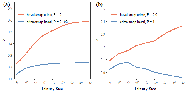
Example of spatial raster data
Load the spEDM package and simulate raster data with a
cyclic interaction structure \(x \rightarrow y
\rightarrow z \rightarrow x\):
if (!requireNamespace("fields")) install.packages("fields")
## Loading required namespace: fields
if (!requireNamespace("MASS")) install.packages("MASS")

sim_trispecies = \(nx,ny,seed = 123){
  grid = expand.grid(seq(0, 10, length.out = nx),
                     seq(0, 10, length.out = ny))
  cov.fun = \(d, range = 1.5, sill=1) sill * exp(-d/range)
  dist.mat = fields::rdist(grid)
  cov.mat = cov.fun(dist.mat, range=1.5, sill=1)
  set.seed(seed)
  res = replicate(3, {
    MASS::mvrnorm(1, rep(0, nrow(grid)), cov.mat) |>
      pmax(0) |>
      sdsfun::normalize_vector(0,1) |>
      matrix(nrow = nx, ncol = ny) |>
      terra::rast()
  }, simplify = FALSE)
  terra::rast(res)
}

species = sim_trispecies(20,20, seed = 42)
names(species) = c("x","y","z")

sim = spEDM::slm(species, x = "x", y = "y", z = "z", k = 4,
                 step = 15, transient = 1, threshold = Inf,
                 aggregate_fn = \(.x) mean(.x, na.rm = TRUE),
                 alpha_x = 0.05, alpha_y = 0.05, alpha_z = 0.05,
                 beta_xy = 1, beta_xz = 0, beta_yx = 0, beta_yz = 1,
                 beta_zx = 1, beta_zy = 0)

terra::values(species[["x"]]) = sim$x
terra::values(species[["y"]]) = sim$y
terra::values(species[["z"]]) = sim$z
species
## class       : SpatRaster
## size        : 20, 20, 3  (nrow, ncol, nlyr)
## resolution  : 1, 1  (x, y)
## extent      : 0, 20, 0, 20  (xmin, xmax, ymin, ymax)
## coord. ref. :
## source(s)   : memory
## names       :         x,         y,        z
## min values  : 0.9984091, 0.9983558, 0.998285
## max values  : 1.0009110, 1.0011445, 1.001050
Determine minimum embedding dimensions:
spEDM::fnn(species, "x")
## [spEDM] Output 'E:i' corresponds to the i-th valid embedding dimension.
## [spEDM] Input E values exceeding max embeddable dimension were truncated.
## [spEDM] Please map output indices to original E inputs before interpretation.
##       E:1       E:2       E:3       E:4       E:5       E:6       E:7       E:8       E:9
## 0.8937824 0.3125000 0.0100000 0.0000000 0.0000000 0.0000000 0.0000000 0.0000000 0.0000000
spEDM::fnn(species, "y")
## [spEDM] Output 'E:i' corresponds to the i-th valid embedding dimension.
## [spEDM] Input E values exceeding max embeddable dimension were truncated.
## [spEDM] Please map output indices to original E inputs before interpretation.
##       E:1       E:2       E:3       E:4       E:5       E:6       E:7       E:8       E:9
## 0.9333333 0.2525000 0.0425000 0.0000000 0.0000000 0.0000000 0.0000000 0.0000000 0.0000000
spEDM::fnn(species, "z")
## [spEDM] Output 'E:i' corresponds to the i-th valid embedding dimension.
## [spEDM] Input E values exceeding max embeddable dimension were truncated.
## [spEDM] Please map output indices to original E inputs before interpretation.
##       E:1       E:2       E:3       E:4       E:5       E:6       E:7       E:8       E:9
## 0.9238845 0.3375000 0.0625000 0.0200000 0.0000000 0.0000000 0.0000000 0.0000000 0.0000000
Self prediction for parameter turning:
s1 = spEDM::simplex(species, "x", "x", E = 5:10, k = 15, tau = 1)
s2 = spEDM::simplex(species, "y", "y", E = 5:10, k = 15, tau = 1)
s3 = spEDM::simplex(species, "z", "z", E = 5:10, k = 15, tau = 1)
list(s1,s2,s3)
## [[1]]
## The suggested E,k,tau for variable x is 7, 15 and 1
##
## [[2]]
## The suggested E,k,tau for variable y is 9, 15 and 1
##
## [[3]]
## The suggested E,k,tau for variable z is 5, 15 and 1
Due to the statistical aggregation performed after simulating with the spatial logistic map, we adopt a uniform embedding dimension for x, y, and z to reduce inference bias:
if (!requireNamespace("purrr")) install.packages("purrr")
## Loading required namespace: purrr
simplex_res = purrr::map2_dfr(list(s1,s2,s3), c("x","y","z"),
                              \(.list,.name) dplyr::mutate(.list$xmap,variable = .name))
ggplot2::ggplot(data = simplex_res) +
  ggplot2::geom_line(ggplot2::aes(x = E, y = rho, color = variable)) +
  ggplot2::theme_classic()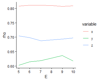
Since the self-prediction performance of the y variable is relatively weaker than that of x and z, we select the embedding dimension that yields the strongest predictive performance for y as the final dimension, that is \(E = 9\).
Investigate the causation between x and z, with y as control variables:
xz = spEDM::scpcm(species, "x", "z", "y", E = 9, k = 15,
                  libsizes = matrix(seq(50,400,50), ncol = 1),
                  progressbar = FALSE)
xz
## --------------------------------------
## ***partial cross mapping prediction***
## --------------------------------------
##   libsizes       x->z      z->x
## 1       50 0.07977338 0.1020714
## 2      100 0.10473775 0.1762694
## 3      150 0.14175015 0.1959109
## 4      200 0.20562278 0.2543825
## 5      250 0.25500417 0.3300376
## 6      300 0.27904324 0.3956866
## 7      350 0.31249554 0.4597477
## 8      400 0.28091955 0.4843444
##
## ------------------------------
## ***cross mapping prediction***
## ------------------------------
##   libsizes      x->z      z->x
## 1       50 0.1542880 0.1368370
## 2      100 0.1827606 0.2217753
## 3      150 0.2426258 0.2781118
## 4      200 0.3239733 0.3487456
## 5      250 0.4035323 0.4185710
## 6      300 0.4653763 0.4835619
## 7      350 0.5190529 0.5553776
## 8      400 0.5658039 0.5938894
Visualize the result:
fig2a = plot(xz,partial = FALSE,ylimits = c(0.05,0.65))
fig2b = plot(xz,partial = TRUE,ylimits = c(0.05,0.65))
fig2 = cowplot::plot_grid(fig2a,fig2b,ncol = 2,label_fontfamily = 'serif',
                          labels = paste0('(',letters[1:2],')'))
fig2